In my third post about advanced log analytics, I want to share a useful technique for analyzing the concurrency of an application based on simple debug logs. Once again, the intended takeaway is that there’s gold hiding even in the simplest debug logs and an advanced log analytics tool is key for the digging. The blog post is entirely based on pre-populated data and script in the Application Insights Analytics demo site so you can experiment hands on with everything you read here.
Some background on concurrency and what we are trying to achieve in this example. Concurrency is about making an app work on multiple tasks simultaneously. Take for example, front end servers that handle interactions with multiple users at the same time. Concurrency is commonly achieved by employing thread pools or by using dedicated asynchronous API (e.g. for querying data from a DB). From a logical perspective, developers usually relate to a sequence of operations that have a beginning and an end in the same context as an activity. The concurrency level of an application is defined as the number of outstanding activities at a given point in time. In other words, it’s the number of activities whose execution is passed the beginning but has not yet reached the end. Highly concurrent applications are more complex by nature than applications with no concurrency. The effective concurrency level of an application is influenced by many factors and has significant effect on the overall behavior and utilization of the other components that interface with the activity (e.g. utilization of a DB is affected by the numbers of concurrent calls by clients). In this example, we will show how simple debug logs can be used to chart the concurrency level of an app over a period in time.
Once again, let’s start by looking at how a single activity is manifested in our debug logs.
let startDate = startofday(datetime("2017-02-01"));
let endDate = startofday(datetime("2017-02-08"));
traces
| where timestamp > startDate and timestamp < endDate
| where operation_Id == "QaXuZhd2b2c="
| project timestamp , operation_Id , message
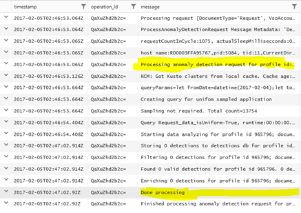
For our example, let’s assume that the interesting part in the logical activity above is the part that starts and ends in the highlighted lines respectively. So next step is to refine our query to keep just these lines. Also, to make our analysis robust, the following lines filter out lines related to activities that don’t have both a beginning and an end in the time range we’re analyzing.
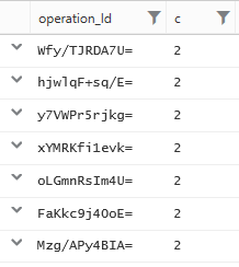
| summarize c = dcount(message) by operation_Id
| where c == 2
The following query generates a list of operation_Ids that are relevant for our analysis.
let startDate = startofday(datetime("2017-02-01"));
let endDate = startofday(datetime("2017-02-08"));
traces
| where timestamp > startDate and timestamp < endDate
| where (message startswith "Processing anomaly detection") or (message == "Done processing")
| project timestamp , message, operation_Id
// Count the distinct message per operation and keep just those that have both a beginning and an end
| summarize c = dcount(message) by operation_Id
| where c == 2
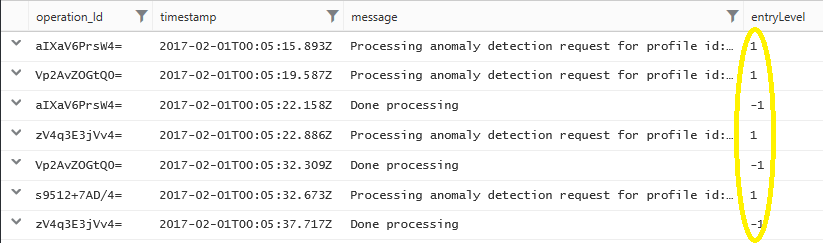
Now that we know which activities we want to keep, let’s apply a self-join to keep just the relevant lines along with the columns of interest. It is a good practice to use materialize() when applying a self-join.
As it is often the case, we want to project our problem into the metric domain. For that, the following query will add a new numeric column with the value 1 to indicate a beginning of an activity and the value -1 to indicate a completion or an end. Since the sequence of the lines is important, the query will order (sort) the records in an ascending order by the timestamp.
let startDate = startofday(datetime("2017-02-01"));
let endDate = startofday(datetime("2017-02-08"));
let T = materialize(
    traces
    | where timestamp > (startDate+1s) and timestamp < endDate
    | where (message startswith "Processing anomaly detection") or (message == "Done processing")
    | project timestamp , message, operation_Id);
T
| summarize c = dcount(message) by operation_Id
| where c == 2
| project operation_Id
| join (T) on operation_Id
| project-away operation_Id1
// Add a numeric column to indicate whether the line represents a beginning or an end
| extend entryLevel = iff(message startswith "Processing", 1, -1)
| order by timestamp asc
In the metric domain again
And here comes the cool part. We can now use infinite impulse response to calculate the cumulative of the numeric entryLevel column. Each term in the cumulative sum indicates the number of outstanding activities (which is what we are looking for) at that specific point in time. Building applicative filters for infinite impulse response requires some understanding in signal processing and is beyond the scope of this blog. So in this example we’re using a predefined sample that wraps the series_iir() function.
series_iir() is a function that takes a time series or an array of dynamic types, so will we will first use makelist() to transpose the output of the previous step into a new table with just one line and two columns. The first column is an ordered array of all the timestamps of all the trace lines and the second column is an array of corresponding numeric indicators (1 / -1) for begin/end of activities. We then extend the table with a third column that is the cumulative sum of the array elements in the 2nd column. Each term in the element array in the 3rd column is in fact the concurrency level of the application in correlation to a timestamp in the same position in the first column. To aggregate these values into a coarser granularity and draw a chart we use mvexpand to transpose once again the single-line table into a multi-line table. We can then apply any type of numeric aggregation and granularity.
// Define a simple function implementing a cumulative sum using Infinite Impulse Response.
let cumsum = (series:dynamic)
{
    series_iir(series, dynamic([1]), dynamic([1,-1]))
};
let startDate = startofday(datetime("2017-02-01"));
let endDate = startofday(datetime("2017-02-08"));
let T = materialize(
    traces
    | where timestamp > (startDate+1s) and timestamp < endDate
    | where (message startswith "Processing anomaly detection") or (message == "Done processing")
    | project timestamp , message, operation_Id);
T
| summarize c = dcount(message) by operation_Id
| where c == 2
| project operation_Id
| join (T) on operation_Id
// Add a numeric column to indicate whether the line represents a beginning or an end
| extend entryLevel = iff(message startswith "Processing", 1, -1)
| order by timestamp asc
// Our cumulative sum function takes arrays and series as parameters, so we'll use makelist() to transpose the table
| summarize timestamp=makelist(timestamp, 1000000), entries=makelist(entryLevel, 1000000)
| extend csum = cumsum(entries)
| project-away entries
// After applying the cumulative sum function, we can now transpose the table back again using mvexpand
| mvexpand timestamp, csum limit 1000000
// Since we can not draw a chart of >300K data points, let's aggregate in 1 minute granularity
| summarize maxConcurrency=max(tolong(csum)) by bin(todatetime(timestamp), 1m)
| project timestamp, maxConcurrency
| render timechart
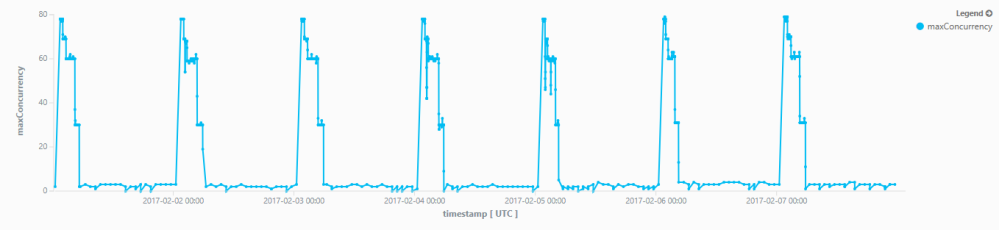
And that’s it
When applied in this sample on 40GB execution logs for ~340K activities of the DeepInsights batch micro service in Application Insights over the course of 7 days, the chart nicely manifests the seasonal daily concurrency level.
